Competing Risks
Hemant Ishwaran
Thomas A. Gerds
Bryan M. Lau
Min Lu
Udaya B. Kogalur
2023-05-29
competing.Rmd
Introduction
Here we outline the extension of random survival forests [1] to competing risks given in [2]. Users should first read the random survival forests vignette [3] if they are unfamiliar with this topic.
In competing risks, unlike survival where there is only one event type, the individual is subject to \(J>1\) competing risks. As in survival data, a complication is that the individual can be right-censored. Formally, let \(T^o\) be the true event time and let \({\delta}^o\in\{1,\ldots,J\}\) record the event type. Let \(C^o\) denote the true censoring time. Under the presence of right-censoring we only observe \(T=\min(T^o,C^o)\) and the censoring indicator \({\delta}={\delta}^o \cdot I\{T^o\le C^o\}\). Thus for each individual one either observes the time an event occurs \(T=T^o\) and the type of event which occured \({\delta}={\delta}^o\in\{1,\ldots,J\}\). Otherwise if the individual is right-censored, we observe the censoring time \(T=C^o\) and the censoring indicator is \({\delta}=0\).
Competing Risk Splitting Rules
There are three splitting rules used by the package to grow a competing risk tree:
Generalized log-rank test, specified by
splitrule = "logrank". This tests for equality of the event-specific hazard and is most appropriate when the analysis focuses on determining factors for event-specific risk. The generalized log-rank test is based on the weighted difference of the Nelson-Aalen event-specific cumulative hazard estimates in the daughter nodes.Gray’s test, specified by
splitrule = "logrankCR"which is the default used by the package. This is a modification of Gray’s test [4] and tests for the equality of the cause-specific cumulative incidence. This is most appropriate when the goal is long term probability prediction.Composite (weighted) splitting. This is specified using
causeand is an integer value between 1 and \(J\) indicating the event of interest for splitting a node, where splitting is either based on the generalized log-rank test or Gray’s test specified bysplitruleas described above. If not specified, the default is to use a composite splitting rule that averages equally over all events. Can also be a vector of non-negative weights of length \(J\) specifying weights for each event (for example, passing a vector of ones reverts to the default composite split-statistic).
Goals of Competing Risks
In competing risks, we are interested in predicting events and discovering risk factors affecting event times. For the latter, we distinguish between risk factors for the cause-specific hazard and risk factors for the cumulative incidence.
The cause-specific hazard function for event \(j=1,\ldots,J\) given a covariate \({\bf X}\) is \[
\alpha_j(t|{\bf X})
= \lim_{\Delta t\rightarrow 0} \frac{\mathbb{P}\{t\le T^o \le t+\Delta t, {\delta}^o=j
| T^o\ge t,{\bf X}\}}{\Delta t}
:= \frac{f_j(t|{\bf X})}{S(t|{\bf X})}.
\] Here \(S(t|{\bf X})=\mathbb{P}\{T^o\ge t|{\bf X}\}\) is the event-free survival probability function given \({\bf X}\). The cause-specific hazard function describes the instantaneous risk of event \(j\) for subjects that currently are event-free. Factors found to change the instantaneous event risk are associated with the biological mechanism behind event \(j\). The logrank split-rule is the appropriate splitting rule to use if the goal focuses on the cause-specific hazard function.
On the other hand, the probability that an event occurs in a specific time period, say \([0,t]\), depends on the cause-specific hazards of the other events [4]. The probability of an event is determined using the cumulative incidence (CIF), defined as the probability of experiencing an event of type \(j\) by time \(t\); i.e. \(F_j(t|{\bf X}) = \mathbb{P}\{T^o \le t, {\delta}^o=j|{\bf X}\}\). The CIF and cause-specific hazard function are related according to \[
F_j(t|{\bf X})
=\int_0^t S(s-|{\bf X})\alpha_j(s|{\bf X})\, d s
= \int_0^t \exp\left(-\int_0^s \sum_{l=1}^J \alpha_l(u|{\bf X})
\, d u\right) \alpha_j(s|{\bf X})\, d s .
\] Informally speaking, event \(j\) can only occur for those surviving other risks. Thus, covariates found to change the \(t\)-year risk of event \(j\) (i.e. the cumulative incidence) are those that change the cause-specific hazard function of event \(j\) and those that change the cause-specific hazard functions of the competing risks. When the goal is \(t\)-year prediction, then the CIF is the appropriate measure and in this case the appropriate splitting rule is logrankCR.
Formal Definition of Splitting Rules
Let \((T_i,{\bf X}_i,\delta_i)_{1\leq i\leq n}\) denote the data where \(T_i\) is the observed time, \(\delta_i\in\{0,1,\ldots,J\}\) is the observed censoring indicator, and \({\bf X}_i\) is the feature. Let \(t_1<t_2<\cdots<t_m\) be the distinct event times. Suppose the proposed split is of the form \(X\le c\) and \(X>c\) for a continuous variable \(X\) (this can be obviously generalized to categorical variables) forming left and right daughters \(L=\{X_i\le c\}\) and \(R=\{X_i>c\}\), respectively. The number of individuals at risk at time \(t\) in the daughter nodes are \[ Y_L(t)=\sum_{i=1}^n I(T_i\ge t,X_i\le c),\hskip10pt Y_R(t)=\sum_{i=1}^n I(T_i\ge t,X_i> c). \] The number of individuals who are risk at time \(t\) is \(Y(t)=Y_L(t)+Y_R(t)\). The number of type \(j\) events at time \(t\) for the left and right daughters is \[ d_{j,L}(t)=\sum_{i=1}^n I(T_i=t, {\delta}_i=j, X_i\le c),\hskip10pt d_{j,R}(t)=\sum_{i=1}^n I(T_i=t, {\delta}_i=j, X_i> c), \] and \(d_j(t)=d_{j,L}(t)+d_{j,R}(t)\) is the total number of type \(j\) events at \(t\), for \(j=1,\ldots,J\).
Generalized Log-Rank Test
The competing risk log-rank test, logrank, is a test of the null hypothesis \(H_{0,j}:\alpha_{j,L}(t)=\alpha_{j,R}(t)\) for all \(t\le\tau\) for some horizon time point \(\tau>0\) where \(\alpha_{J,l}, \alpha_{j,R}\) are the cause-\(j\) specific hazard rates in the left and the right daughter nodes.
The test is based on the difference of the Nelson-Aalen cause-specific cummulative hazard function estimate in the two daughter nodes. Specifically, for the split at the value \(c\) for variable \(X\), the splitrule is
(1)
\[ L^{\mathrm{LR}}_j(X,c) =\frac 1{\hat\sigma^{\mathrm{LR}}_{j}(X,c)}\sum_{k=1}^m\left(d_{j,L}(t_k) -\frac{d_j(t_k)Y_L(t_k)}{Y(t_k)}\right) \] where the variance estimate is given by \[ (\hat\sigma^{\mathrm{LR}}_{j}(X,c))^{2}= \sum_{k=1}^m d_j(t_k) \frac{Y_L(t_k)}{Y(t_k)} \left(1-\frac{Y_L(t_k)}{Y(t_k)}\right) \left(\frac{Y(t_k)-d_j(t_k)}{Y(t_k)-1}\right). \] Note that time-dependent weights \(w_j(t_k)>0\) can be used to make the test more sensitive to early or late differences between the cause-specific hazards [2]. The choice \(w_j(t_k)=1\) used implicitly here (and which is adopted in the package) corresponds to the standard log-rank test which has optimal power for detecting alternatives where the cause-specific hazards are proportional. The best split is found by maximizing \(|L_{j}^{\mathrm{LR}}(X,c)|\) over \(X\) and \(c\).
If the aim is to identify variables that are important for any cause, it can be useful to combine the cause-specific splitting rules across the event types, i.e. \(H_{0,j}\) for \(j=1,\ldots,J\), which is accomodated by using the composite split-statistic \[
L^{\mathrm{LR}}(X,c)
= \frac{\sum_{j=1}^J W_j \hat\sigma^{\mathrm{LR}}_j(X,c)
L_j^{\mathrm{LR}}(X,c)}{\sqrt{\sum_{j=1}^JW_j^2(\hat\sigma^{\mathrm{LR}}_j(X,c))^2}}.
\] By default, the package assumes that this is the case and assigns constant weights \(W_j=1\) to all events, \(j=1,\ldots,J\). In order to focus on a specific event, say \(j\), and only test \(H_{0,j}:\alpha_{j,L}(t)=\alpha_{j,R}(t)\), users can do so by using the option cause. For example, cause=1 or cause=c(1,0,0) would focus on event \(j=1\) in a setting where \(J=3\). One can also specify different weights for the events, for example cause=c(4,1,1) places a weight four times larger on event \(j=1\).
Gray’s Test
If the goal is prediction of cumulative event probabilities, then it is more appropriate to construct a test statistic to test for differences in the CIF. The split-rule logrankCR does this and is modeled after Gray’s test [4], which tests the null hypothesis \(H_{0,j}:F_{j,L}(t)=F_{j,R}(t)\) for all \(t\le \tau\) where \(F_{j,L}, F_{j,R}\) are the CIF’s for the left and right daughters.
Technical details of the modified Gray’s split-statistic are given in [2]. The package implements a special version of this test statistic which modifies the risk set in the log-rank test statistic. For example, the risk set \(Y(t)\) in equation (1) is replaced by the modified risk set \[ Y^*_j(t) = \sum_{i=1}^n I\Bigl(T_i\ge t \cup \left(T_i< t \cap {\delta}_i\ne j \cap {\delta}_i\ne 0\right)\Bigr). \] This equals the number of individuals who have not had an event prior to \(t\) in addition to those individuals who have experienced an event \(j'\ne j\) prior to \(t\), but who are not censored. A similar change is made to the risk set \(Y_L(t)\) appearing in equation (1). The split-statistic is denoted by \(L_j^{\mathrm{G}}(X,c)\).
By default, the package implements an omnibus test of equality of all CIF’s simultaneously by using a composite split-rule \[
L^{\mathrm{G}}(X,c)
= \frac{\sum_{j=1}^J W_j \hat\sigma^{\mathrm{G}}_j(X,c)
L_j^{\mathrm{G}}(X,c)}{\sqrt{\sum_{j=1}^JW_j^2(\hat\sigma^{\mathrm{G}}_j(X,c))^2}}
\] where \((\hat\sigma^{\mathrm{G}}_{j}(X,c))^{2}\) is the variance estimate for the event \(j\) test. Similar to log-rank splitting, the package assigns constant weights \(W_j=1\) to all events which can be over-ridden using the option cause.
Event-Specific Terminal Node Statistics (TNS)
Let \(n_{i,b}\) be the number of times case \(i\) occurs in the bootstrap sample of the \(b\)th tree. Let \(h_b({\bf X})\) be the terminal node of the \(b\)th tree containing \({\bf X}\). Denote IB (in-bag) node-specific event counts by \[ N_{j,b}^{\text{IB}}(t|{\bf X})=\sum_{i\in h_b({\bf X})}n_{i,b}I\{T_i\leq t, \delta_i=j\}, \quad{}j=1,\ldots,J \] and IB number at risk by \[ Y_b^{\text{IB}}(t|{\bf X})=\sum_{i\in h_b({\bf X})}n_{i,b}I\{T_i\geq t\}. \]
Cumulative Incidence Function: The tree estimator for \(F_j(t|{\bf X})\) is the Aalen-Johansen [5] tree estimator \[ F_{j,b}^{\text{IB}}(t|{\bf X}) =\int_{(0,t]}S_b^{\text{IB}}(u-|{\bf X}) Y_b^{\text{IB}}(u|{\bf X})^{-1}N_{j,b}^{\text{IB}}(du|{\bf X}), \quad{}j=1,\ldots,J, \] where \[ S_b^{\text{IB}}(t|{\bf X})=\prod_{u\leq t}\left[1-\sum_{j=1}^J \frac{N_{j,b}^{\text{IB}}(du|{\bf X})}{Y_b^{\text{IB}}(u|{\bf X})}\right] \] is the Kaplan-Meier tree estimate of the event-free survival function, \(S(t|{\bf X})\).
Cumulative Hazard Function: The tree estimator for the event-specific cumulative hazard function \(H_j(t|{\bf X})=\int_0^t \alpha_j(u|{\bf X}) du\) is the Nelson-Aalen tree estimator \[ H_{j,b}^{\text{IB}}(t|{\bf X}) = \int_0^t Y_b^{\text{IB}}(u|{\bf X})^{-1}N_{j,b}^{\text{IB}}(du|{\bf X}). \]
Event-Specific Ensembles
Tree-averaging \(F_{j,b}^{\text{IB}}(t|{\bf X})\) yields the IB ensemble estimate for the event-specific CIF \[ \bar{F}_j^{\text{IB}}(t|{\bf X})=\frac{1}{\texttt{ntree}}\sum_{b=1}^\texttt{ntree} F_{j,b}^{\text{IB}}(t|{\bf X}), \quad{}j=1,\ldots,J. \] Let \(O_i\) record trees where case \(i\) is OOB (out-of-bag). The OOB ensemble estimator for case \(i\) is \[ \bar{F}_{i,j}^{\text{OOB}}(t)=\frac{1}{|O_i|}\sum_{b\in O_i}F_{j,b}^{\text{IB}}(t|{\bf X}_i), \quad{}j=1,\ldots,J. \] Likewise, IB and OOB ensemble estimators for the event-specific cumulative hazard function are \[ \bar{H}_j^{\text{IB}}(t|{\bf X})=\frac{1}{\texttt{ntree}}\sum_{b=1}^\texttt{ntree} H_{j,b}^{\text{IB}}(t|{\bf X}),\hskip15pt \bar{H}_{i,j}^{\text{OOB}}(t)=\frac{1}{|O_i|}\sum_{b\in O_i} H_{j,b}^{\text{IB}}(t|{\bf X}_i). \]
Expected Number of Life Years Lost (Cause-\(j\) Mortality)
The predicted value used by the package for competing risks is the one-dimensional summary of the cumulative incidence refered to as the expected number of life years lost due to cause \(j\) [6]. In right-censored data it is not feasible to get a reliable estimate of the expected lifetime. Therefore for a fixed time point \(\tau\) we consider the restricted mean lifetime conditional on \({\bf X}\) \[ R_{\text{MLT}}({\bf X})=\int_0^\tau S(t|{\bf X})\, d t. \] In practice, the package sets \(\tau\) to the maximum observed event time, \(t_m\). We extend the notation of [6] to the case with covariates and note the relation \(S(t|{\bf X})+\sum_{j=1}^J F_j(t|{\bf X})=1\). The expected number of years lost before time \(\tau\) for \({\bf X}\) is \[ \tau - R_{\text{MLT}}({\bf X}) =\tau-\int_0^\tau S(t|{\bf X})\,d t = \int_0^\tau \sum_{j=1}^J F_j(t|{\bf X})\, d t. \] Our summary value is \(M_j(\tau|{\bf X}) = \int_0^\tau F_j(t|{\bf X})\, dt\), which the above shows equals the expected number of life years lost due to cause \(j\) before time \(\tau\). We shall also call \(M_j(\tau|{\bf X})\) the cause-\(j\) mortality. This value is estimated by replacing \(F_j\) with the IB ensemble estimator \(\bar{F}_j^{\text{IB}}(t|{\bf X})\). For the purposes of prediction error estimation it is replaced with the OOB estimator, yielding OOB expected number of life years lost for an individual \(i\) \[ \bar{M}_{i,j}^{\text{OOB}}(\tau) = \int_0^\tau \bar{F}_{i,j}^{\text{OOB})}(t)\, dt, \quad{}j=1,\ldots,J. \]
Illustration
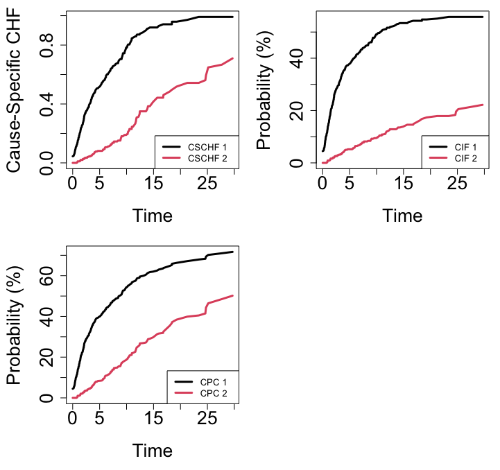
As a first illustration, we use the follicular cell lymphoma data from [7]. The subset of 541 patients includes all patients identified as having follicular type lymphoma. Patients were treated with radiation alone or with radiation and chemotherapy. The two types of events are relapse (\(j=1\)) and death (\(j=2\)) and the data is subect to right censoring. Figure 1 displays the averaged OOB ensemble CSCHF (cause-specific CHF), CIF and continuous probability curves (CPC) for each event [8] from a forest grown using the default composite Gray splitting rule.
Variable Importance Illustration
In our second illustration, we show how applying different splitting rules can be used for variable importance analysis in competing risks. To illustrate, we use the Mayo Clinic Primary Biliary Cirrhosis (PBC) data from [9]. The data consists of a subset of 312 cases having mostly complete data from the original 424 patient cohort, as well as an additional 106 cases collected later. There are \(J=2\) events: death (\(j=1\)) and transplant (\(j=2\)) and the data is subject to right censoring. There are a total of \(p=17\) features.
We run three different analyses. Missing data was eliminated for simplicity. Analysis 1 uses the default logrankCR split-statistic and tests whether the CIF is equal for the two events of death and transplant. Analysis 2 uses the logrank split-statistic and is used for assessing variable importance for the case-specific event of death. The option cause=c(1,0) is used to accomplish this. Analysis 3 is similar to Analysis 2, but assesses variable importance for transplant events. The option cause=c(0,1) is used to accomplish this.
For assessing variable importance in Analysis 1, we extract the minimal depth [10] from its forests. In this context, small minimal depth values indicate variables that affect \(t\)-years prediction for all events. Minimal depth and variable importance values are given in the output. Overall, “bili” is the most important variable and affects both types of events. The variable “age” is highly event-specific and primarily affects death.
Note importantly that when extracting VIMP from Analyses 2 and 3, we were careful to only extract VIMP for the targeted specific event. Thus for Analysis 2, this is column one of VIMP, which corresponds to death, whereas for Analysis 3, it is column two, which corresponds to transplant.
library("randomForestSRC")
## illustrates the various CR splitting rules
## illustrates event specific and non-event specific variable selection

## load the survival package
library("survival")

## use the pbc data where events are death (1) and transplant (2)
data(pbc, package = "survival")
pbc$id <- NULL

## Analysis 1
## modified Gray's weighted log-rank splitting
## (equivalent to cause=c(1,1) and splitrule="logrankCR")
o1 <- rfsrc(Surv(time, status) ~ ., pbc, ntree = 1000)

## Analysis 2
## log-rank cause-1 (death) specific splitting and targeted VIMP
o2 <- rfsrc(Surv(time, status) ~ ., pbc,
                  splitrule = "logrank", cause = c(1,0), importance = TRUE)

## Analysis 3
## log-rank cause-2 (transplant) specific splitting and targeted VIMP
o3 <- rfsrc(Surv(time, status) ~ ., pbc,
                  splitrule = "logrank", cause = c(0,1), importance = TRUE)

## extract VIMP from the log-rank forests: event-specific
## extract minimal depth from the Gray log-rank forest: non-event specific
vimpOut <- data.frame(md = max.subtree(o1)$order[, 1],
                      vimp.death = 100 * o2$importance[ ,1],
                      vimp.transplant = 100 * o3$importance[ ,2])

print(vimpOut[order(vimpOut$md), ], digits = 2)

>           md vimp.death vimp.transplant
> bili     2.0     7.0377          6.4049
> copper   3.4     1.4955          1.8384
> albumin  4.2    -0.7029          0.8055
> edema    4.2    -0.0471          1.2472
> protime  4.6     0.1441          0.6063
> ascites  4.6     0.0341          1.1718
> chol     5.0     0.3578          0.4316
> age      5.2     7.5407          0.8018
> ast      5.6     0.0098          0.3986
> alk.phos 5.9    -0.6136          0.1632
> stage    6.0     0.6931          0.3928
> trig     6.2    -0.6467          0.1096
> platelet 6.3     1.3386         -0.0517
> hepato   6.7     0.5715          0.0652
> spiders  7.3    -0.1343          0.1191
> sex      7.4    -0.0667          0.0114
> trt      7.9    -0.2518          0.0092
Cite this vignette as
H. Ishwaran, T. A. Gerds, B. M. Lau, M. Lu, and U. B. Kogalur. 2021. “randomForestSRC: competing risks vignette.” http://randomforestsrc.org/articles/competing.html.
@misc{HemantCompeting,
    author = "Hemant Ishwaran and Thomas A. Gerds and Bryan M. Lau and Min Lu and Udaya B. Kogalur",
    title = {{randomForestSRC}: competing risks vignette},
    year = {2021},
    url = {http://randomforestsrc.org/articles/competing.html},
    howpublished = "\url{http://randomforestsrc.org/articles/competing.html}",
    note = "[accessed date]"
}